
March 13, 2014 From rOpenSci (https://ropensci.org/blog/2014/03/13/rnoaa/). Except where otherwise noted, content on this site is licensed under the CC-BY license.
We recently pushed the first version of rnoaa to CRAN - version 0.1. NOAA has a lot of data, some of which is provided via the National Climatic Data Center, or NCDC. NOAA has provided access to NCDC climate data via a RESTful API - which is great because people like us can create clients for different programming languages to access their data programatically. If you are so inclined to write a bit of R code, this means you can get to NCDC data in the R environment where your workflow is reproducible, and you can connect data acquisition to a suite of tools for data manipulation (e.g., plyr), visualization (e.g., ggplot2), and statistics (e.g., lme4, etc.).
In addition to NCDC climate data, we have functions to access sea ice cover data via FTP, as well as the Severe Weather Data Inventory (SWDI) via API. We will continue to add in other data sources as we have time.
Some notes:
- The docs for the API are live at the NOAA NCDC website
- GCHN Daily data is also available via FTP.
The below examples uses the development version, but most things can be done with the CRAN version. Here’s a quick run down of some things you can do with rnoaa:
🔗 First, install and load taxize
install.packages("rnoaa")
or development version from GitHub
install.packages("devtools")
library(devtools)
install_github("rnoaa", "ropensci")
library(rnoaa)
library(rnoaa)
🔗 API keys - authentication
You’ll need an API key to use this package (essentially a password). Go to the NCDC website to get one. You can’t use this package without an API key.
Once you obtain a key, there are two ways to use it.
a) Pass it inline with each function call (somewhat cumbersome and wordy)
noaa(datasetid = "PRECIP_HLY", locationid = "ZIP:28801", datatypeid = "HPCP",
    limit = 5, token = "YOUR_TOKEN")
b) Alternatively, you might find it easier to set this as an option, either by adding this line to the top of a script or somewhere in your .Rprofile file
options(noaakey = "KEY_EMAILED_TO_YOU")
Specifically use the name noaakey as the functions in the rnoaa package are looking for a key by that name.
🔗 Fetch list of city locations in descending order
noaa_locs(locationcategoryid = "CITY", sortfield = "name", sortorder = "desc",
    limit = 5)
## $meta
## $meta$totalCount
## [1] 1654
##
## $meta$pageCount
## [1] 5
##
## $meta$offset
## [1] 1
##
##
## $data
##              id           name datacoverage    mindate    maxdate
## 1 CITY:NL000012     Zwolle, NL       1.0000 1892-08-01 2014-01-31
## 2 CITY:SZ000007     Zurich, SZ       1.0000 1901-01-01 2014-03-11
## 3 CITY:NG000004     Zinder, NG       0.8678 1906-01-01 1980-12-31
## 4 CITY:UP000025  Zhytomyra, UP       0.9726 1938-01-01 2014-03-11
## 5 CITY:KZ000017 Zhezkazgan, KZ       0.9279 1948-03-01 2014-03-10
##
## attr(,"class")
## [1] "noaa_locs"
🔗 Get info on a station by specifcying a dataset, locationtype, location, and station
noaa_stations(datasetid = "GHCND", locationid = "FIPS:12017", stationid = "GHCND:USC00084289")
## $meta
## NULL
##
## $data
##                  id                  name datacoverage    mindate
## 1 GHCND:USC00084289 INVERNESS 3 SE, FL US            1 1899-02-01
##      maxdate
## 1 2014-03-12
##
## attr(,"class")
## [1] "noaa_stations"
🔗 Search for data
out <- noaa(datasetid = "GHCND", stationid = "GHCND:USW00014895", datatypeid = "PRCP",
    startdate = "2010-05-01", enddate = "2010-10-31")
🔗 See a data.frame
head(out$data)
##             station value attributes datatype                date
## 1 GHCND:USW00014895     0  T,,0,2400     PRCP 2010-05-01T00:00:00
## 2 GHCND:USW00014895    30   ,,0,2400     PRCP 2010-05-02T00:00:00
## 3 GHCND:USW00014895    51   ,,0,2400     PRCP 2010-05-03T00:00:00
## 4 GHCND:USW00014895     0  T,,0,2400     PRCP 2010-05-04T00:00:00
## 5 GHCND:USW00014895    18   ,,0,2400     PRCP 2010-05-05T00:00:00
## 6 GHCND:USW00014895    30   ,,0,2400     PRCP 2010-05-06T00:00:00
🔗 Get table of all datasets
res <- noaa_datasets()
res$data
##                     uid         id                    name datacoverage
## 1  gov.noaa.ncdc:C00040     ANNUAL        Annual Summaries         1.00
## 2  gov.noaa.ncdc:C00861      GHCND         Daily Summaries         1.00
## 3  gov.noaa.ncdc:C00841    GHCNDMS       Monthly Summaries         1.00
## 4  gov.noaa.ncdc:C00345    NEXRAD2         Nexrad Level II         0.95
## 5  gov.noaa.ncdc:C00708    NEXRAD3        Nexrad Level III         0.95
## 6  gov.noaa.ncdc:C00821 NORMAL_ANN Normals Annual/Seasonal         1.00
## 7  gov.noaa.ncdc:C00823 NORMAL_DLY           Normals Daily         1.00
## 8  gov.noaa.ncdc:C00824 NORMAL_HLY          Normals Hourly         1.00
## 9  gov.noaa.ncdc:C00822 NORMAL_MLY         Normals Monthly         1.00
## 10 gov.noaa.ncdc:C00505  PRECIP_15 Precipitation 15 Minute         0.25
## 11 gov.noaa.ncdc:C00313 PRECIP_HLY    Precipitation Hourly         1.00
##       mindate    maxdate
## 1  1831-02-01 2013-11-01
## 2  1763-01-01 2014-03-13
## 3  1763-01-01 2014-01-01
## 4  1991-06-05 2014-03-12
## 5  1994-05-20 2014-03-09
## 6  2010-01-01 2010-01-01
## 7  2010-01-01 2010-12-31
## 8  2010-01-01 2010-12-31
## 9  2010-01-01 2010-12-01
## 10 1970-05-12 2013-03-01
## 11 1900-01-01 2013-03-01
🔗 Get data category data and metadata
noaa_datacats(locationid = "CITY:US390029", limit = 5)
## $meta
## $meta$totalCount
## [1] 37
##
## $meta$pageCount
## [1] 5
##
## $meta$offset
## [1] 1
##
##
## $data
##        id                 name
## 1  ANNAGR  Annual Agricultural
## 2   ANNDD   Annual Degree Days
## 3 ANNPRCP Annual Precipitation
## 4 ANNTEMP   Annual Temperature
## 5   AUAGR  Autumn Agricultural
##
## attr(,"class")
## [1] "noaa_datacats"
🔗 Plotting
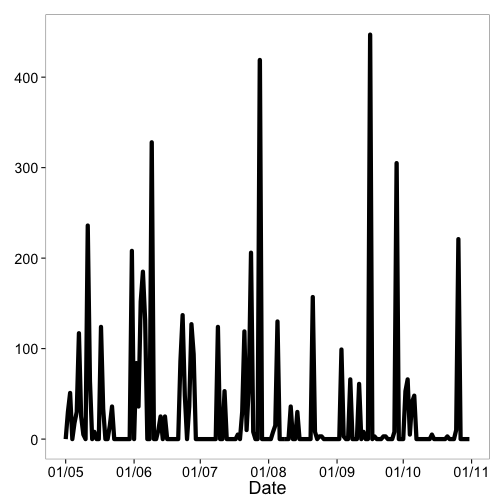
🔗 Plot data, super simple, but it’s a start
out <- noaa(datasetid = "GHCND", stationid = "GHCND:USW00014895", datatypeid = "PRCP",
    startdate = "2010-05-01", enddate = "2010-10-31", limit = 500)
noaa_plot(out, breaks = "1 month", dateformat = "%d/%m")
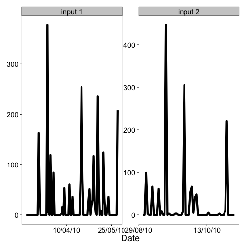
🔗 More plotting
You can pass many outputs from calls to the noaa function in to the noaa_plot function.
out1 <- noaa(datasetid = "GHCND", stationid = "GHCND:USW00014895", datatypeid = "PRCP",
    startdate = "2010-03-01", enddate = "2010-05-31", limit = 500)
out2 <- noaa(datasetid = "GHCND", stationid = "GHCND:USW00014895", datatypeid = "PRCP",
    startdate = "2010-09-01", enddate = "2010-10-31", limit = 500)
noaa_plot(out1, out2, breaks = "45 days")
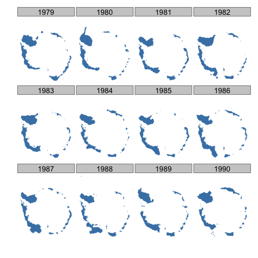
🔗 Sea ice cover data
Get urls for ftp files
urls <- sapply(seq(1979, 1990, 1), function(x) seaiceeurls(yr = x, mo = "Feb",
    pole = "S"))
Call the noaa_seaice function on each url, which downloads shape files, and reads them in to R as sp objects
out <- lapply(urls, noaa_seaice)
Then plot
library(plyr)
library(ggplot2)
names(out) <- seq(1979, 1990, 1)
df <- ldply(out)
ggplot(df, aes(long, lat, group = group)) + geom_polygon(fill = "steelblue") +
    theme_ice() + facet_wrap(~.id)
🔗 Severe weather data
🔗 Search for nx3tvs data from 5 May 2006 to 6 May 2006
noaa_swdi(dataset = "nx3tvs", startdate = "20060505", enddate = "20060506",
    limit = 3)
## $meta
## $meta$totalCount
## [1] 3
##
## $meta$totalTimeInSeconds
## [1] 0.004
##
##
## $data
##                  ztime wsr_id cell_id cell_type range azimuth max_shear
## 1 2006-05-05T00:05:50Z   KBMX      Q0       TVS     7     217       403
## 2 2006-05-05T00:10:02Z   KBMX      Q0       TVS     5     208       421
## 3 2006-05-05T00:12:34Z   KSJT      P2       TVS    49     106        17
##   mxdv
## 1  116
## 2  120
## 3   52
##
## $shape
##                                        shape
## 1 POINT (-86.8535716274277 33.0786326913943)
## 2 POINT (-86.8165772540846 33.0982820681588)
## 3 POINT (-99.5771091971025 31.1421609654838)
##
## attr(,"class")
## [1] "noaa_swdi"
🔗 Get all ‘plsr’ within the bounding box (-91,30,-90,31)
noaa_swdi(dataset = "plsr", startdate = "20060505", enddate = "20060510", bbox = c(-91,
    30, -90, 31), limit = 3)
## $meta
## $meta$totalCount
## [1] 3
##
## $meta$totalTimeInSeconds
## [1] 0.015
##
##
## $data
##                  ztime     id        event magnitude         city
## 1 2006-05-09T02:20:00Z 427540         HAIL         1 5 E KENTWOOD
## 2 2006-05-09T02:40:00Z 427536         HAIL         1 MOUNT HERMAN
## 3 2006-05-09T02:40:00Z 427537 TSTM WND DMG     -9999 MOUNT HERMAN
##       county state          source
## 1 TANGIPAHOA    LA TRAINED SPOTTER
## 2 WASHINGTON    LA TRAINED SPOTTER
## 3 WASHINGTON    LA TRAINED SPOTTER
##
## $shape
##                  shape
## 1 POINT (-90.43 30.93)
## 2  POINT (-90.3 30.96)
## 3  POINT (-90.3 30.96)
##
## attr(,"class")
## [1] "noaa_swdi"
🔗 Get all ‘nx3tvs’ within the tile -102.1/32.6
noaa_swdi(dataset = "nx3tvs", startdate = "20060506", enddate = "20060507",
    tile = c(-102.12, 32.62), limit = 3)
## $meta
## $meta$totalCount
## [1] 3
##
## $meta$totalTimeInSeconds
## [1] 0.021
##
##
## $data
##                  ztime wsr_id cell_id cell_type range azimuth max_shear
## 1 2006-05-06T00:41:29Z   KMAF      D9       TVS    37       6        39
## 2 2006-05-06T03:56:18Z   KMAF      N4       TVS    39       3        30
## 3 2006-05-06T03:56:18Z   KMAF      N4       TVS    42       4        20
##   mxdv
## 1   85
## 2   73
## 3   52
##
## $shape
##                                        shape
## 1 POINT (-102.112726356403 32.5574494581267)
## 2  POINT (-102.14873079873 32.5933553250156)
## 3 POINT (-102.131167022161 32.6426287452898)
##
## attr(,"class")
## [1] "noaa_swdi"
🔗 Counts
Get number of ‘nx3tvs’ within 15 miles of latitude = 32.7 and longitude = -102.0
noaa_swdi(dataset = "nx3tvs", startdate = "20060505", enddate = "20060516",
    radius = 15, center = c(-102, 32.7), stat = "count")
## $meta
## $meta$totalCount
## [1] 1
##
## $meta$totalTimeInSeconds
## [1] 0.02
##
##
## $data
## [1] "37"
##
## $shape
## data frame with 0 columns and 1 rows
##
## attr(,"class")
## [1] "noaa_swdi"
